Classification🔗

Documentation : https://spark.apache.org/docs/latest/ml-classification-regression.html

Use Cases🔗

predicting potential credit default risk while lending (Binary Classification)
categorizing news posts or article based on their content
using sensors based data on a smart watch to determine physical activity

Types of Classification🔗

Binary Classification🔗

only two labels to predict, example: detecting whether an email is spam or not

Multiclass Classification🔗

choose a label from multiple labels, example: facebook predicting people in a given photo, meterological prediction for weather

Multilabel Classification🔗

choose mutilple labels, exmaple: predict a book’s genre from the text of book, could belong to multiple genre

Classification Models in MLlib🔗

Spark has several models available for performing binary and multiclass classification out of the box.

Spark does not support making multilabel predictions natively. In order to train a multilabel model, you must train one model per label and combine them manually

Model Scalability🔗

Model scalability is a very important metric while choosing a model, Spark performs good on large-scale machine learning models but there on a single-node workloads there are number of tools that will outperform spark.

Model	Features count	Training examples	Output classes
Logistic regression	1 to 10 million	No limit	Features x Classes < 10 million
Decision trees	1,000s	No limit	Features x Classes < 10,000s
Random forest	10,000s	No limit	Features x Classes < 100,000s
Gradient-boosted trees	1,000s	No limit	Features x Classes < 10,000s

Data for classification models

bInput = spark.read.format("parquet").load("/data/binary-classification")\
  .selectExpr("features", "cast(label as double) as label")

Logistic Regression🔗

very popular regression methods for classification. It is linear method that combines individual features with specific weights that combined to get a probability of belonging to a class.
Weights represents the importance of a features

Model Hyperparameters🔗

family : can be multinomial (two or more distinct labels) or binary (only two labels)
elasticNetParam : A float value (0, 1) which specifies the mix of L1 and L2 regularization according to elastic net regularization. L1 regularization will create sparsity in model because features weights will become zero (that are little consequence to output). L2 regularization doesn’t create sparsity because corresponding weights for a particular features will only be driven towards zero, but will never reach zero.
fitIntercept : Boolean value, determines whether to fit the intercept or the arbitrary number that is added to the linear combination of inputs and weights of the model. Typically you will want to fit the intercept if we haven’t normalized our training data.
regParam : A value >= 0. that determines how much weight to give to regularization term in objective function. Choosing a value here is again going to be a function of noise and dimensionality in our dataset.
standardization : Boolean Value deciding whether to standardize inputs before passing them into the models.

Training Parameters🔗

maxIter : Total number of iterations over the data before stopping. Default is 100.
tol : specifies a threshold by which changes in parameters show that we optimized our weights enough, and can stop iterating. It lets the algorithm stop before maxIter iteration. Default is : 1e-6
weightCol : name of weight column used to weigh certain rows more than other

Prediciton Parameters🔗

threshold : A Double in the range 0 to 1. This parameter is probability threshold for when a given class should be predicted. You can tune this parameter to your requirements to balance between false positives and false negatives. For instance, if a mistake prediction is very costly, set this to very high value.
thresholds : This parameter lets you specify an array of threshold values for each class when using multiclass classification.

Example🔗

To get all params

from pyspark.ml.classification import LogisticRegression
lr = LogisticRegression()
print lr.explainParams() # see all parameters
lrModel = lr.fit(bInput)

once model is trained we can get information about model by taking a look at intercepts and coefficients. The coefficients correspond to the individual feature weights while the intercept is the value of the italics-intercept.

print(lrModel.coefficients)
print(lrModel.intercept)

For a multinomial model (the current one is binary), lrModel.coefficientMatrix and lrModel.interceptVector can be used to get the coefficients and intercept. These will return Matrix and Vector types representing the values or each of the given classes.

Model Summary🔗

Logistic regression provides a model summary that gives you information about the final, trained model.

Using the summary, we can get all sorts of information about the model itself including the area under the ROC curve, the f measure by threshold, the precision, the recall, the recall by thresholds, and the ROC curve. Note that for the area under the curve, instance weighting is not taken into account, so if you wanted to see how you performed on the values you weighed more highly, you’d have to do that manually.

Decision Trees🔗

more friendly and interpretable models for performing classification because similar to decision models that resembles human decision use.

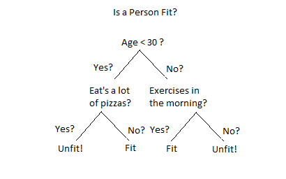
In short you create a big decision tree to predict the outcomes, this model supports multiclass classifications as well.
Although this model is good start, it does come at a cost. It can overfit data extremely quickly. Unrestrained this decision tree will create a pathway from start based on every training example.
This is bad because then the model won’t generalize to new data (you will see poor test set prediction performance). However, there are a number of ways to try and rein in the model by limiting its branching structure (e.g., limiting its height) to get good predictive power.

Model Hyperparameters🔗

maxDepth: specifies max depth in order to avoid overfitting dataset
maxBins: In decision trees, continuous features are converted into categorical features and maxBins determines how many bins should be created from continous features. More bins gives a higher level of granularity. The value must be greater than or equal to 2 and greater than or equal to the number of categories in any categorical feature in your dataset. The default is 32
impurity : To build a “tree” you need to configure when the model should branch. Impurity represents the metric to determine whether or not model should splits at a particular leaf node. This parameter can be set to either be “entropy” or “gini” (default), two commonly used impurity metrics
minInfoGain : this param determines the minimum information gain that can be used for a split. A higher value can prevent overfitting. This is largely something that needs to be determines from testing out different variations of the decision tree model. Ddefault : 0
minInstancePerNode : This parameter determines the minimum number of training instances that need to end in a particular node. Think of this as another manner of controlling max depth. We can prevent overfitting by limiting depth or we can prevent it by specifying that at minimum a certain number of training values need to end up in a particular leaf node. If it’s not met we would “prune” the tree until that requirement is met. A higher value can prevent overfitting. The default is 1, but this can be any value greater than 1.

Training Parameters🔗

checkpointInterval : Checkpointing is a way to save the model’s work over the course of training so that if nodes in cluster crash for some reason, we don’t lose our work. This parameter needs to be set together with a checkpointDir (a directory to checkpoint to) and with useNodeIdCache=true

Prediction Parameters🔗

There is only one prediction parameters for decision trees : thresholds

from pyspark.ml.classification import DecisionTreeClassifier
dt = DecisionTreeClassifier()
print dt.explainParams()
dtModel = dt.fit(bInput)

Random Forest and Gradient-Boosted Trees🔗

This method is an extension of decision tree which trains multiple trees on varying subsets of data. Each of those trees become expert in a particular domain relevant to subset picked and we combine them to get a concensus. These methods help preventing overfitting.
Random forests and gradient-boosted trees are two distinct methods for combining decision trees. In random forests we simply train lots of trees and then average their response to make a prediction. With gradient-boosted trees, each tree makes a weighted prediction. They have largely same parameters stated below.
One current limitation is that gradient-boosted trees currently only support binary labels. There are several popular tools for learning tree-based models. For example, the XGBoost library provides an integration package for Spark that can be used to run it on Spark.

Model Hyperparameters🔗

Both support all same model hyperparameters as decision trees.

Random forest only🔗

numTrees : total number of trees to train
featureSubsetStrategy : determines how many features should be considered for splits. This can be a variety of different values including “auto”, “all”, “sqrt”, “log2”, or a number “n.” When your input is “n” the model will use n * number of features during training.

Gradient-boosted trees (GBT) only🔗

lossType: loss function for gradient-boosted trees to minimize during training. Currently, only logistic loss is supported.
maxIter : Total number of iterations over the data before stopping. Changing this probably won’t change your results a ton, so it shouldn’t be the first parameter you look to adjust. The default is 100.
stepSize : This is the learning rate for the algorithm. A larger step size means that larger jumps are made between training iterations. This can help in the optimization process and is something that should be tested in training. The default is 0.1 and this can be any value from 0 to 1.

Training Parameters🔗

checkpointInterval

Prediction Parameters🔗

Have same prediction parameters as decision trees.

Examples

# RF Tree
from pyspark.ml.classification import RandomForestClassifier
rfClassifier = RandomForestClassifier()
print rfClassifier.explainParams()
trainedModel = rfClassifier.fit(bInput)

# GBT Tree
from pyspark.ml.classification import GBTClassifier
gbtClassifier = GBTClassifier()
print gbtClassifier.explainParams()
trainedModel = gbtClassifier.fit(bInput)

Naive Bayes🔗

Naive Bayes classifiers are a collection of classifiers based on Bayes’ theorem. The core assumption behind the models is that all features in your data are independent of one another. Naturally, strict independence is a bit naive, but even if this is violated, useful models can still be produced.
Naive Bayes classifiers are commonly used in text or document classification, although it can be used as a more general-purpose classifier as well.
There are two different model types:
- either a multivariate Bernoulli model, where indicator variables represent the existence of a term in a document;
- or the multinomial model, where the total counts of terms are used.
One important note when it comes to Naive Bayes is that all input features must be non-negative.

Model Hyperparameters🔗

modelType: Either “bernoulli” or “multinomial”
weightCol : Allows weighing different data points differently.

Training Parameters🔗

smoothing : This determines the amount of regularization that should take place using additive smoothing. This helps smooth out categorical data and avoid overfitting on the training data by changing the expected probability for certain classes. The default value is 1.

Prediction Parameters🔗

Naive Bayes shares the same prediction parameter, thresholds

from pyspark.ml.classification import NaiveBayes
nb = NaiveBayes()
print nb.explainParams()
trainedModel = nb.fit(bInput.where("label != 0"))

Evaluators for Classification and Automating Model Tuning🔗

Evaluator on its doesn’t help too much, unless we use it in a pipeline, we can automate a grid search of our various parameters of models and transformers - trying all combinations of parameters to see which ones perform best.
For classification, there are two evaluators, and they expect two columns: a predicted label from the model and a true label.
For binary classification we use the BinaryClassificationEvaluator. This supports optimizing for two different metrics “areaUnderROC” and areaUnderPR.”
For multiclass classification, we need to use the MulticlassClassificationEvaluator, which supports optimizing for “f1”, “weightedPrecision”, “weightedRecall”, and “accuracy”.

Detailed Evaluation Metrics🔗

MLlib also contains tools that let you evaluate multiple classification metrics at once. Unfortunately, these metrics classes have not been ported over to Spark’s DataFrame-based ML package from the underlying RDD framework. Check documentation for more information

There are 3 different Classifications metrics we can use

Binary classification metrics
Multiclass classification metrics
Multilabel classification metrics

from pyspark.mllib.evaluation import BinaryClassificationMetrics
out = model.transform(bInput)\
  .select("prediction", "label")\
  .rdd.map(lambda x: (float(x[0]), float(x[1])))
metrics = BinaryClassificationMetrics(out)

print metrics.areaUnderPR
print metrics.areaUnderROC
print "Receiver Operating Characteristic"
metrics.roc.toDF().show()

One-vs-Rest Classifier🔗

There are some MLlib models that don’t support multiclass classification. In these cases, users can leverage a one-vs-rest classifier in order to perform multiclass classification given only a binary classifier.
The intuition behind this is that for every class you hope to predict, the one-vs-rest classifier will turn the problem into a binary classification problem by isolating one class as the target class and grouping all of the other classes into one.
One-vs-rest is implemented as an estimator. For the base classifier it takes instances of the classifier and creates a binary classification problem for each of the 𝘬 classes. The classifier for class i is trained to predict whether the label is i or not, distinguishing class i from all other classes.
Predictions are done by evaluating each binary classifier and the index of the most confident classifier is output as the label.
See spark documentation for more.

Multilayer Perceptron🔗

The multilayer perceptron is a classifier based on neural networks with a configurable number of layers (and layer sizes). We will discuss it in 3 chapters ahead